Example usage ecm clustering

Here we will demonstrate how to use evclust to make an evidential clustering with the iris dataset. Assuming that there is uncertainty in the species data and that there may be species in several clusters at once or in none at all

import evclust

print(evclust.__version__)

0.2.1

Imports

from evclust.ecm import ecm
from evclust.datasets import load_decathlon, load_iris
from evclust.utils import ev_summary, ev_plot, ev_pcaplot

Matplotlib is building the font cache; this may take a moment.

Data

There is test data in the package. Here we’re going to use the popular IRIS data

# Import test data
df = load_iris()
df=df.drop(['species'], axis = 1) # del label column
df.head()

	sepal_length	sepal_width	petal_length	petal_width
0	5.1	3.5	1.4	0.2
1	4.9	3.0	1.4	0.2
2	4.7	3.2	1.3	0.2
3	4.6	3.1	1.5	0.2
4	5.0	3.6	1.4	0.2

ECM

# Evidential clustering with c=3
from evclust.ecm import ecm
model = ecm(x=df, c=3, beta = 2,  alpha=1, delta=10)

[1, np.float64(39.91648998781675)]
[2, np.float64(39.581085891128566)]
[3, np.float64(39.50696993719648)]
[4, np.float64(39.45417364896527)]
[5, np.float64(39.403940855534714)]
[6, np.float64(39.35140469150919)]
[7, np.float64(39.29479315388693)]
[8, np.float64(39.23414217104631)]
[9, np.float64(39.170981591784766)]
[10, np.float64(39.1080026711019)]

[11, np.float64(39.04842832901853)]
[12, np.float64(38.99517100495034)]
[13, np.float64(38.950120428619755)]
[14, np.float64(38.91387055476747)]
[15, np.float64(38.88591248640273)]
[16, np.float64(38.86507245133501)]
[17, np.float64(38.849943636847996)]
[18, np.float64(38.83917952903764)]
[19, np.float64(38.83163705826829)]
[20, np.float64(38.82641427367434)]

[21, np.float64(38.822832210970745)]
[22, np.float64(38.82039550336568)]
[23, np.float64(38.81875036822346)]
[24, np.float64(38.81764790810152)]
[25, np.float64(38.81691493063716)]

Read and Summary the output

We can summary the output of the ecm model, to see Focal sets or Number of outliers

ev_summary(model)

------ Credal partition ------
3 classes,
150 objects
Generated by ecm
Focal sets:
[[0. 0. 0.]
 [1. 0. 0.]
 [0. 1. 0.]
 [1. 1. 0.]
 [0. 0. 1.]
 [1. 0. 1.]
 [0. 1. 1.]
 [1. 1. 1.]]
Value of the criterion = 38.82
Nonspecificity = 0.22
Prototypes:
[[4.96375502 3.3462016  1.49213248 0.24695422]
 [6.01335287 2.76720722 4.77762377 1.64225065]
 [7.06131634 3.03675091 6.05972886 2.1474559 ]]
Number of outliers = 0.00

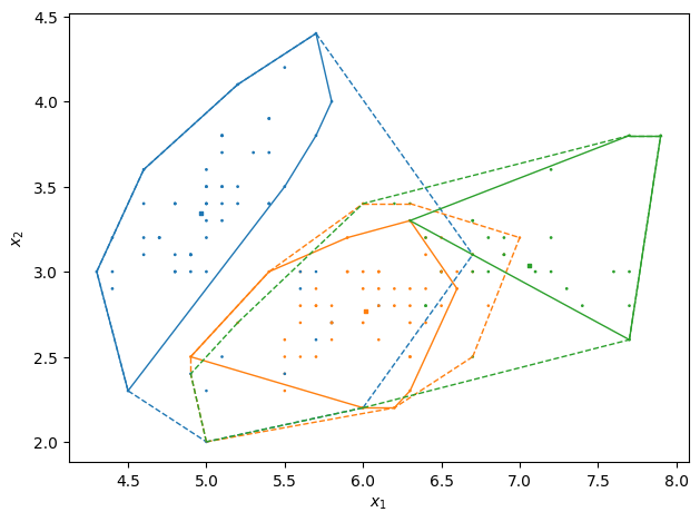
Plot the creadal partition

We can now plot the result based on the two features axes using ev_plot function

ev_plot(x=model,X=df)